How do customers feel about our product? What are the public sentiments regarding the latest news about COVID-19? How positive or negative are the prevailing impressions regarding a particular politician?
Traditional approaches to answering these questions have involved conducting surveys and polls of relevant populations. Nowadays, these inquiries can also be addressed by examining online platforms where public sentiments are abundant.
Analyzing public sentiments can be challenging due to the volume of data generated over time. On Twitter alone, users post thousands of tweets each second.
Hence, it would be prohibitively time-consuming to inspect every tweet manually. This challenge has created a demand for methods, such as sentiment analysis algorithms, capable of mining these data in an automated fashion.
Sentiment analysis elucidates the underlying emotions expressed in a given text. These can include positive, negative, or even neutral sentiments. In practice, it can be hard to train a model to identify emotions given their subjective nature.
However, to meet this challenge, natural language processing techniques have been devised to extract numerical features from written text. These features are used to train machine learning models to identify sentiments.
In this post, I will describe a simple way to train a binary classifier to perform sentiment analysis.
I first learned this technique in the Natural Language Specialization course on Coursera. I will test this approach on a dataset, found on Kaggle, containing customer reviews from Amazon. Here, I am going to outline the steps I took to prepare this data for machine learning.
I will also examine the performance of a linear support vector machine (SVM) sentiment classifier. This model was trained to classify the sentiments of the reviews in this dataset and achieved a classification accuracy of 75% on my testing set.
Contents#
- A Simple Technique For Classifying Sentiment
- Performing Sentiment Analysis on a Dataset of Amazon Product Reviews
- Some Additional Considerations
- Conclusion
A Simple Technique For Classifying Sentiment#
Carl Sagan noted that to make an apple pie from scratch, you must first invent the universe. Correspondingly, it goes without saying that to train a machine learning model you first need to acquire data, which unfortunately is not as impressive as inventing the universe.
Start by preparing a dataset that contains text samples with corresponding labels denoting their sentiment. In my case, each customer review had either a positive or negative sentiment label.
After preparing a dataset, partition the data into two parts: a training set used to train our model and a testing set used to evaluate our model’s performance. The main challenge now is to extract relevant features to train a sentiment classifier.
Using the training set, we can construct two features. For a given sample of text, compute the sum of how often each word in the text appears in the text samples in the training set labeled as having a positive sentiment.
This sum will serve as the first feature for our model. The second feature will be derived from a similar procedure. This time, compute the sum of how often each word in appears within the text samples in the training set that have a negative sentiment. The following expression defines these features:
where represents the -th word in the given sample text. The first component of this vector represents the sum of the positive frequencies of each word. The second component corresponds to the sum of the negative frequencies of each word.
Let’s see how to implement this in some code. For this, I will use the Natural Language Toolkit (NLTK), a well-established library for natural language processing. I’m going to import a few functions from this library:
import nltk
nltk.download('punkt')
from nltk.tokenize import word_tokenize
from nltk.probability import FreqDist
Here, the function word_tokenize takes a string as input and generates a list of words in the given string. Each item in this list is known as a word token.
Furthermore, the FreqDist function takes these word tokens and generates a dictionary where the keys consist of each unique token. The corresponding values are the frequencies of each token.
Finally, the line containing nltk.download(‘punkt’) downloads the Punkt module which is the default tokenizer function used by word_tokenize. Here’s an example showing how these two functions can be used together:
sample_text = "the quick brown fox jumps over the lazy dog"
FreqDist(word_tokenize(sample_text))
Running this code outputs the following dictionary showing how often each word occurs in sample_text:
FreqDist({'the': 2, 'quick': 1, 'brown': 1, 'fox': 1,
		  'jumps': 1, 'over': 1, 'lazy': 1, 'dog': 1})
This example illustrates one of the key steps needed to construct numerical features for sentiment analysis. Using the training set, we will have to perform this process to obtain two dictionaries showing how often a word occurs in the positive reviews and the negative reviews, respectively.
I’ve defined the function get_freqdists to generate these two dictionaries containing the positive frequencies pos_freqs, and the negative frequencies neg_freqs. The input for this function is assumed to be a DataFrame with two columns. These include review_text which contains the text from each review, and sentiment which contains corresponding sentiment labels for each review.
def get_freqdists(dataset):
    def get_freqs(dataset):
        total_text = dataset["review_text"].to_list()
        total_text = " ".join(total_text)
        word_tokens = word_tokenize(total_text)
        return FreqDist(word_tokens)

    pos_dataset = dataset.loc[dataset["sentiment"] == "positive"]
    neg_dataset = dataset.loc[dataset["sentiment"] == "negative"]

    pos_freqs = get_freqs(pos_dataset)
    neg_freqs = get_freqs(neg_dataset)

    return pos_freqs, neg_freqs
Once we have the dictionaries containing the positive and negative frequencies of the words in our training set, we can write another function to generate the features for a given text sample.
I have defined the function get_features for this purpose. Using the input_text, it computes a feature vector containing the sums of the positive and negative frequencies of the words contained in the text.
def get_features(input_text, pos_freqs, neg_freqs):
    pos_count = 0
    neg_count = 0

    word_lst = word_tokenize(input_text)
    for word in word_lst:
        if word in pos_freqs:
            pos_count += pos_freqs[word]

        if word in neg_freqs:
            neg_count += neg_freqs[word]

    return [pos_count, neg_count]
I will demonstrate how these functions work in the following example. Let’s start by defining a small dataset containing customer product reviews:
import pandas as pd

dataset = pd.DataFrame({"review_text": ["Best product ever!",
                                        "Much excite. Such wow!",
                                        "Not happy with this product.",
                                        "Very bad, this product was."],
                       "sentiment": ["positive",
                                     "positive",
                                     "negative",
                                     "negative"]})
dataset
This dataset is represented by the table below:
| review_text | sentiment | |
|---|---|---|
| 0 | Best product ever! | postive |
| 1 | Much excite. Such wow! | postive |
| 2 | Not happy with this product. | negative |
| 3 | Very bad, this product was. | negative |
Before we begin, we will have to pre-process this text. The steps for this are:
- Remove all punctuation marks and stop words.
- Convert all characters to lowercase.
- Stem each word
We remove punctuation marks as these don’t directly correlate with the sentiment of a text. It is also typically recommended to remove stop words for this same reason. These include words such as “is”, “was”, “of”, “but”, “very”, and many others.
Next, we lowercase each word so that capitalized words aren’t treated as being distinct from their lowercase counterparts.
Finally, we convert each word to its corresponding stem, a process known as stemming. For example, the words “going”, “goes”, and “gone” are derived from the stem word “go.” Stemming ensures that we don’t count each of these words separately as they all carry the same lexical meaning.
The function clean_text defined below implements these pre-processing steps. Here, I’ve imported some additional definitions from the nltk library. These include the PorterStemmer class used for stemming each word, and stopwords which is a list of stop words. I also imported the string library as string.puncutation contains the punctuation marks we will need to remove from each text sample.
nltk.download('stopwords')
from nltk.stem import PorterStemmer
from nltk.corpus import stopwords
import string

def clean_text(text):
    table = str.maketrans('', '', string.punctuation)
    new_text = text.translate(table)

    new_text = new_text.lower()
    word_lst = word_tokenize(new_text)

    output = []
    stemmer = PorterStemmer()
    for word in word_lst:
        if word in stopwords.words('english'):
            continue
        else:
            word = stemmer.stem(word)
            output.append(word)

    return " ".join(output)
We can clean each of the text entries by executing the following:
dataset.loc[:, "review_text"] = dataset.loc[:, "review_text"].apply(
    lambda x: clean_text(x)
)
dataset
After running this, the dataset now looks like:
| review_text | sentiment | |
|---|---|---|
| 0 | best product ever | postive |
| 1 | much excit wow | postive |
| 2 | happi product | negative |
| 3 | bad product | negative |
There are a few things to note about the processed text.
For instance, the words “happy” and “excite” have been modified to become “happi” and “excit,” respectively. These are the word stems identified by the PorterStemmer algorithm.
Also, some of the original words in the reviews are missing because stop words were removed. In particular, the first negative review that was “not happy with this product” became “happi product.” Here, “not” is a stop word that negated the word “happy,” giving this review a negative sentiment.
Because this stop word was deleted, the review now appears to have a positive sentiment. Nuances such as this represent one of the shortcomings of this approach as it ignores negations that are crucial to identifying the conveyed sentiment.
Now, we can construct frequency dictionaries for the positive and negative reviews using the get_freqdists function:
pos_freqs, neg_freqs = get_freqdists(dataset)

pos_freq_table = pd.DataFrame.from_dict(pos_freqs, orient="index")
pos_freq_table.columns = ["pos_freqs"]

neg_freq_table = pd.DataFrame.from_dict(neg_freqs, orient="index")
neg_freq_table.columns = ["neg_freqs"]

freq_table = pos_freq_table.merge(
    neg_freq_table, how="outer", left_index=True, right_index=True
)

freq_table = freq_table.fillna(0)
freq_table
The frequency dictionaries are represented in freq_table, shown in the table below:
| pos_freqs | neg_freqs | |
|---|---|---|
| bad | 0.0 | 1.0 |
| best | 1.0 | 0.0 |
| ever | 1.0 | 0.0 |
| excit | 1.0 | 0.0 |
| happi | 0.0 | 1.0 |
| much | 1.0 | 0.0 |
| product | 1.0 | 2.0 |
| wow | 1.0 | 0.0 |
This table lists each unique word in the dataset. It also shows how often each word appears in the positive reviews and the negative reviews. These are denoted as pos_freqs and neg_freqs, respectively. For instance, the word “product” appeared twice in the negative reviews and only appeared once in the positive reviews.
Now, we can use the get_features function to derive a feature vector for any given review.
text = "very good product love it"
text = clean_text(text)
text, get_features(text, pos_freqs, neg_freqs)('good product love', [1, 2])This code shows the cleaned text along with its feature vector. The words “very” and “it” were removed because they are stop words. Furthermore, the word “product” is the only word in this review that appears in either the positive or negative reviews in the training set.
This word had a frequency of 1 in the positive reviews and a frequency of 2 in the negative reviews. That explains why its feature vector has these frequencies as its components.
In summary, construct numerical features for sentiment analysis using the method I’ve described involves the following:
- Pre-process the text for each review
- Create positive and negative frequency dictionaries using reviews from the training set
- For a given review, sum over the positive frequencies of each word contained in the review. Then, compute a second sum over the negative frequencies of each word.
Performing Sentiment Analysis on a Dataset of Amazon Product Reviews#
When I first learned about this approach to sentiment analysis, I was curious about how well it would work in practice. To address this curiosity, I found a dataset on Kaggle that contains a few million Amazon customer reviews.
This dataset includes two files: train.ft.txt and test.ft.txt that correspond to the training and testing sets, respectively. Within these text files, each sample has the following format:
__label__[X] [review text goes here]In other words, each product review is preceded by a class label. This label could either be __label__1 that represents 1- and 2-star reviews, or __label__2 that represents 4- and 5-star reviews.
According to the documentation, the dataset doesn’t include 3-star reviews. One additional detail is that some of the reviews are written in other languages such as Spanish, although most are in English.
Loading the Dataset#
I began by opening the text file containing the training data. Because this file contains millions of reviews, I loaded 20 samples to briefly examine some of these.
f = open("./train.ft.txt", 'r')
num_samples = 20
lines_lst = []

for i in range(num_samples):
    lines_lst.append(f.readline())

for i in range(4):
    print(lines_lst[i])
Executing the code above reads the file train.ft.txt and prints out the first 4 reviews which are shown below:
'__label__2 Stuning even for the non-gamer: This sound track was beautiful! It paints the senery in your mind so well I would recomend it even to people who hate vid. game music! I have played the game Chrono Cross but out of all of the games I have ever played it has the best music! It backs away from crude keyboarding and takes a fresher step with grate guitars and soulful orchestras. It would impress anyone who cares to listen! ^_^\n'

"__label__2 The best soundtrack ever to anything.: I'm reading a lot of reviews saying that this is the best 'game soundtrack' and I figured that I'd write a review to disagree a bit. This in my opinino is Yasunori Mitsuda's ultimate masterpiece. The music is timeless and I'm been listening to it for years now and its beauty simply refuses to fade.The price tag on this is pretty staggering I must say, but if you are going to buy any cd for this much money, this is the only one that I feel would be worth every penny.\n"

__label__2 Amazing!: This soundtrack is my favorite music of all time, hands down. The intense sadness of "Prisoners of Fate" (which means all the more if you've played the game) and the hope in "A Distant Promise" and "Girl who Stole the Star" have been an important inspiration to me personally throughout my teen years. The higher energy tracks like "Chrono Cross ~ Time's Scar~", "Time of the Dreamwatch", and "Chronomantique" (indefinably remeniscent of Chrono Trigger) are all absolutely superb as well.This soundtrack is amazing music, probably the best of this composer's work (I haven't heard the Xenogears soundtrack, so I can't say for sure), and even if you've never played the game, it would be worth twice the price to buy it.I wish I could give it 6 stars.

__label__2 Excellent Soundtrack: I truly like this soundtrack and I enjoy video game music. I have played this game and most of the music on here I enjoy and it's truly relaxing and peaceful.On disk one. my favorites are Scars Of Time, Between Life and Death, Forest Of Illusion, Fortress of Ancient Dragons, Lost Fragment, and Drowned Valley.Disk Two: The Draggons, Galdorb - Home, Chronomantique, Prisoners of Fate, Gale, and my girlfriend likes ZelbessDisk Three: The best of the three. Garden Of God, Chronopolis, Fates, Jellyfish sea, Burning Orphange, Dragon's Prayer, Tower Of Stars, Dragon God, and Radical Dreamers - Unstealable Jewel.Overall, this is a excellent soundtrack and should be brought by those that like video game music.Xander Cross
Most of the initial reviews were for a soundtrack for the game Chrono Cross. I’ve never listened to this soundtrack before or played Chrono Cross but I must say I was intrigued by these reviews!
After glancing through the reviews, I could tell that this dataset would need some cleaning. Some reviews had misspelled words.
Here, I thought about whether to correct spelling mistakes although I opted not to implement this in the end. I also noticed that sometimes there wasn’t whitespace after certain punctuation marks like periods.
This was important to note since my clean_text function defined earlier would convert a string such as “two.words” to twowords after removing punctuation marks. Here, I implicitly assumed that there would always be whitespace before or after each punctuation mark.
Preprocessing the Inputs#
I wrote two functions to obtain the sentiment labels and the corresponding text from the file containing the data.
Here, I noticed that the 10th character, indexed as line[9], was the sentiment label that could be 1 (1- and 2-star reviews) or 2 (4- and 5-star reviews).
Furthermore, the 11th character was always whitespace. The characters after this were just the review text.
def get_labels(lines_lst):
    return [line[9] for line in lines_lst]

def get_review_text(lines_lst):
    return [line[11:] for line in lines_lst]
I used the load_dataset function shown below to load a specified number of reviews from a given input file. Here, I modified the sentiment labels 1 and 2 to become negative and positive, respectively.
I also added a regular expression to add a space after periods and commas. This procedure ensured that words separated by these punctuation marks wouldn’t become merged after cleaning the text.
import re

def load_dataset(input_file, num_samples):

    f = open(input_file, 'r')
    lines_lst = []

    for i in range(num_samples):
        lines_lst.append(f.readline())

    labels = get_labels(lines_lst)
    review_text = get_review_text(lines_lst)

    dataset = pd.DataFrame({"review_text": review_text, "sentiment":labels})
    dataset.loc[:, "sentiment"] = dataset["sentiment"].replace(
        {"1": "negative", "2": "positive"}
    )
    dataset.loc[:, "review_text"] = dataset["review_text"].map(
        lambda x: re.sub(r'(?<=[.,])(?=[^\s])', r' ', x)
    )
    dataset.loc[:, "review_text"] = dataset["review_text"].map(
        lambda x: clean_text(x)
    )

    return dataset
I then defined another function get_ml_dataset to prepare the dataset for machine learning. This function takes the DataFrame dataset of the labeled reviews. It generates the matrix X containing the features of each review and the vector y that contains the corresponding sentiment labels for each review.
import numpy as np

def get_ml_dataset(dataset, pos_freqs, neg_freqs):
    text = dataset["review_text"].to_list()
    X = [get_features(text, pos_freqs, neg_freqs) for text in train_text]
    X = np.array(X)
    y = dataset["sentiment"].to_list()
    return X, y
Next, I loaded the first 5000 reviews in the file containing the training data.
train_data_file = "./train.ft.txt"
train_data = load_dataset(train_data_file, 5000)
train_data
These are some of the reviews in the training set:
| review_text | sentiment | |
|---|---|---|
| 0 | stune even nongam sound track beauti paint sen… | positive |
| 1 | best soundtrack ever anyth im read lot review … | positive |
| 2 | amaz soundtrack favorit music time hand intens… | positive |
| 3 | excel soundtrack truli like soundtrack enjoy v… | positive |
| 4 | rememb pull jaw floor hear youv play game know… | positive |
| … | … | … |
| 4995 | must read anyon interest true crime rivet last… | positive |
| 4996 | sheer mad meticul document ye review correct e… | positive |
| 4997 | weirdest plot ever true rememb last year aroun… | positive |
| 4998 | excit book ive ever read love thought book mag… | positive |
| 4999 | book scare hell vincent bugliosi isnt kid writ… | positive |
Then, I loaded some of reviews from the testing set.
test_data_file = "./test.ft.txt"
test_data = load_dataset(test_data_file, 1000)
These are some of the reviews in the testing set:
| review_text | sentiment | |
|---|---|---|
| 0 | great cd love pat great voic gener listen cd y… | positive |
| 1 | best game music soundtrack game didnt realli p… | positive |
| 2 | batteri die within year bought charger jul 200… | negative |
| 3 | work fine maha energi better check maha energi… | positive |
| 4 | great nonaudiophil review quit bit combo playe… | positive |
| … | … | … |
| 995 | borinmg dumb wast time glori old time movi tri… | negative |
| 996 | best film year best film ever made god monster… | positive |
| 997 | see movi ian mckellen perform god monster supe… | positive |
| 998 | best screenplay stabil recent film anticip goo… | positive |
| 999 | tree arriv bent poorli pack manufactur pack pr… | negative |
As a quick check, I wanted to see whether the classes in the training set were balanced so I wrote the following function for this purpose. Compared to the testing set, the training set was very imbalanced. It had 2308 positive reviews and 2692 negative reviews.
def get_label_count(dataset):
    num_pos = len(dataset.loc[dataset["sentiment"] == "positive"])
    num_neg = len(dataset.loc[dataset["sentiment"] == "negative"])
return num_pos, num_neg>>>get_label_count(train_data), get_label_count(test_data)
((2308, 2692), (502, 498))To address this, I wrote the following function to create a training set with equal numbers of positive and negative reviews:
def balance_data(dataset):
    pos_data = train_data.loc[train_data["sentiment"] == "positive"]
    neg_data = train_data.loc[train_data["sentiment"] == "negative"]

    if len(pos_data) > len(neg_data):
        pos_data = pos_data.sample(len(neg_data))
    elif len(pos_data) < len(neg_data):
        neg_data = neg_data.sample(len(pos_data))

    return pd.concat([pos_data, neg_data])
I now created a new balanced dataset bal_train_data and used this to generate the positive and negative frequency dictionaries.
bal_train_data = balance_data(train_data)
pos_freqs, neg_freqs = get_freqdists(bal_train_data)
Training a Linear Model to Classify Sentiments#
Now for the fun part! I first generated the matrices containing features for the training set and testing set along with vectors containing the sentiment labels for each review. I also used the StandardScaler class from the scikit-learn library to standardize each feature.
from sklearn.preprocessing import StandardScaler
scaler = StandardScaler()
X_train, y_train = get_ml_dataset(bal_train_data, pos_freqs, neg_freqs)
X_train = scaler.fit_transform(X_train)
X_test, y_test = get_ml_dataset(test_data, pos_freqs, neg_freqs)
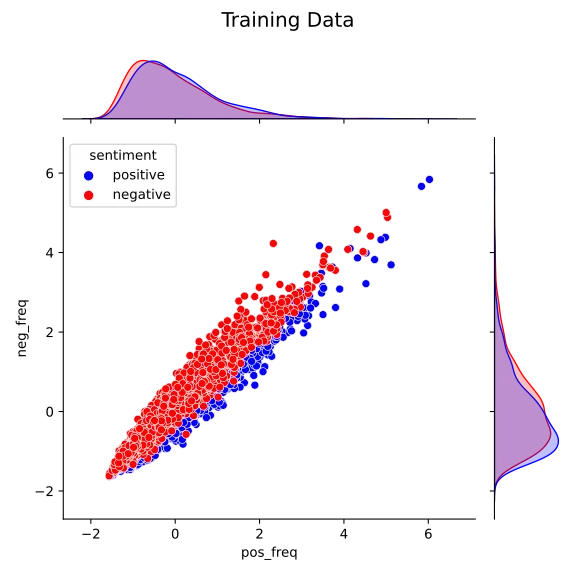
X_test = scaler.transform(X_test)Next, I plotted the features of each review in the training set. For this purpose, I used the library seaborn. The plotting functions defined in this library only take Dataframes. Hence, I created a new DataFrame containing the features from the training set reviews.
import seaborn as sns

ml_train_data_df = pd.DataFrame(data=X_train, columns=["pos_freq", "neg_freq"])
ml_train_data_df.loc[:, "sentiment"] = y_train
ml_train_data_df

jg = sns.jointplot(data=ml_train_data_df,
              x="pos_freq",
              y="neg_freq",
              hue="sentiment",
              palette={"positive": "blue", "negative": "red"})

jg.fig.suptitle("Training Data", size=15)
jg.fig.tight_layout()
jg.fig.subplots_adjust(top=0.9)
After creating the plot shown below, I noted that the two features were correlated. This finding suggested that many words in the frequency dictionaries occurred at equal frequencies in the positive and in the negative reviews. It was also clear that it would be challenging to discriminate between positive and negative reviews using these features.
I also plotted the testing set. This plot bore some similarities with that of the training set. In particular, the same correlation between pos_freq and neg_freq was present.
ml_test_data_df = pd.DataFrame(data=X_test, columns=["pos_freq", "neg_freq"])
ml_test_data_df.loc[:, "sentiment"] = y_test

jg = sns.jointplot(data=ml_test_data_df,
              x="pos_freq",
              y="neg_freq",
              hue="sentiment",
              palette={"positive": "blue", "negative": "red"})

jg.fig.suptitle("Testing Data", size=15)
jg.fig.tight_layout()
jg.fig.subplots_adjust(top=0.9)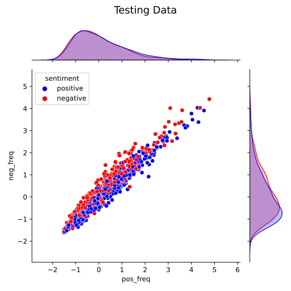
Next, I fitted a linear SVM classifier on the training dataset and scored its performance. The SVM achieved a classification accuracy of 77.9% on the training data.
from sklearn.svm import LinearSVC

lin_svm = LinearSVC(dual=False)
lin_svm.fit(X_train, y_train)
lin_svm.score(X_train, y_train)
#0.7796793760831889
The real test now was to see how the model would perform on the testing set. Here, I observed a classification accuracy of 75% shown below.
>>>lin_svm.score(X_test, y_test)
0.75
I plotted two confusion matrices using the training and testing sets to examine the classification performance further.
from sklearn.metrics import plot_confusion_matrix
plot_confusion_matrix(lin_svm, X_train, y_train)
plt.title("Confusion Matrix: Training Data\n")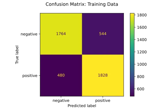
plot_confusion_matrix(lin_svm, X_test, y_test)
plt.title("Confusion Matrix: Testing Data\n")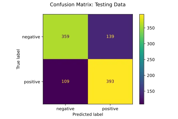
The confusion matrices suggested that the model wasn’t biased toward predicting one sentiment more frequently than the other. Furthermore, the small gap between the model’s performance on the training and testing sets suggests that model isn’t overfitting to the training data.
Some Additional Considerations#
There are more things I could have done to clean the data further.
In cleaning the data, I didn’t correctly handle contracted words. Based on how I processed the text, the string “I’d” would become “id”.
I also noticed spelling mistakes in some of the reviews. For this, I initially used the library pyspellchecker to correct spelling mistakes. But I later decided not to use it as it added a significant amount of time to the pre-processing step.
I also didn’t take into account that some reviews weren’t in English. Here, I could have used the library polyglot to detect the language of each review. This would ensure that my training and testing sets wouldn’t have reviews written in other languages.
Conclusion#
In this post, I described a simple method to generate two numerical features for sentiment analysis. This method requires a training set containing text samples labeled as having either a positive or negative sentiment.
For any text sample, the first feature represents the total sum of how often each word in the text occurs in the training set samples labeled as positive. The second feature represents the sum of the frequencies that each word occurs in training set samples labeled as negative.
I demonstrated this approach using a dataset of Amazon customer reviews. Here, I trained a linear SVM sentiment classifier that achieved a prediction accuracy of 75% on my testing set.